ABSTRACT
Although plugins like Kuka PRC, Robots have enabled robot path simulation on Grasshopper for milling, they haven’t tackled the pre-fabrication milling visualization from a stock, which is crucial to troubleshooting any issues in milling before any physical resources like the workpiece material, machine or the tool are invested. This project aimed to serve as a visualization tool based on voxel collision-detection. The algorithm takes the same time to compute, no matter how large the geometries being voxelized are.
PSEUDO-CODE
The programme was implemented using Python libraries in Grasshopper. The algorithm is divided into three distinct steps as below:
- Voxelization
- Create a bounding-box of the workpiece geometry
- Divide the box into points at distances of the “voxel-size”
- Determine voxels lie inside the workpiece geometry
- Collision-Detection
- Check for collision detection at a time “t”(0<t<T) of the simulation.
- Label the voxels which collide with the tool-geometry as “1”
- Display
- Output the voxels labeled as “0”.
PART 1: VOXELIZATION
Voxelization refers to converting a 3D-model into a set of discrete points to represent the geometry in the space. This is done by creating a bounding-box outside the workpiece geometry. This domain of the box is divided into equidistant points in X, Y and Z directions. Each of this points is checked if they lie within the workpiece geometry.
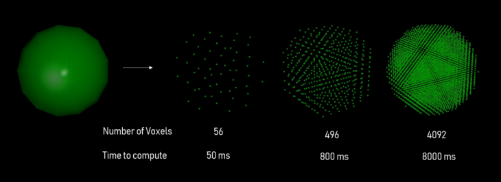 Figure 1. Voxelization of a sphere
Greater the number of voxels, the more realistic it appears like the original geometry. However, the computation time it takes to calculate the coordinates and display them as points increase linearly with the number of voxels. Hence, the voxel resolution value is a trade-off against visual clarity and the algorithm run-time.
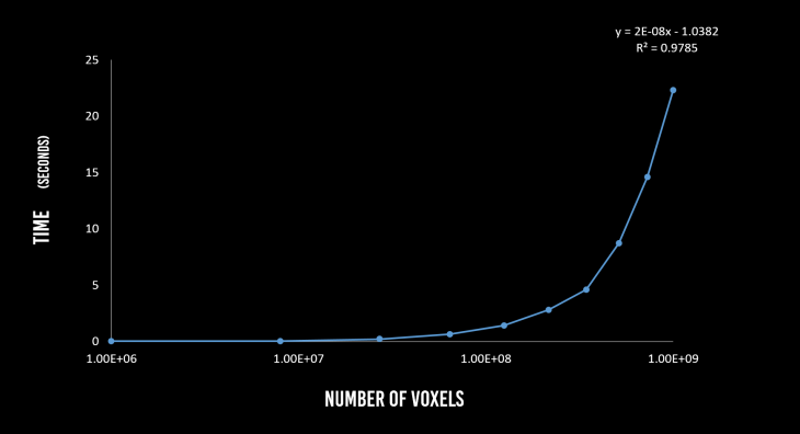 Figure 2. Voxelization algorithm run-time as a function of the number of voxels
PART 2: COLLISION-DETECTION
Once the workpiece geometry is voxelized, the next step is to check which of the voxels collide or lie inside the tool-geometry at any given time. If it does, that particular voxel is deleted from the 3D list containing all the voxels. However, this method requires checking each voxel whether it lies inside the too-geometry at any instant. This is not a scalable approach because if the number of increases a thousandfold, the time to check increases them increases by the same factor.
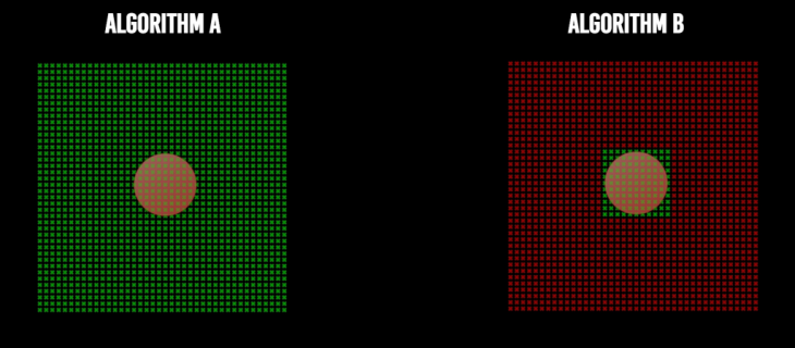 Figure 3. Voxel number invariant collision-detection
Instead, an advantage from the physical workspace dictates the development of a second algorithm. The fact that the milling tool is always smaller than the workpiece geometry is used to compute the indices of voxels in the 3D list which lie in the domain of the tool geometry. Then the same collision-detection algorithm is run on just these indices. Thus, no matter how many voxels there are to check, for the same voxel resolution, the algorithm only checks for the same number of voxels dictated by the dimensions of the tool (cylinder) as shown in Figure 3.
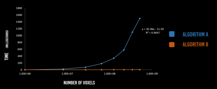 Figure 4. Collision-Detection algorithm run-time as a function of the number of voxels. Algorithm A checks all voxels while B depends on tool-domain
This voxel number invariant collision-detection ensures that the run-time of the algorithm remains the same (approximately 5ms) as the number of voxels increase.
PART 3: DISPLAY
The last step after computation involves displaying the “remaining” voxels in the Rhino viewport. This step scales linearly as the number of voxels increase. However, due to the difference in the time of computation for collision detection using the two algorithms, the slopes of the lines vary as shown in Figure 5.
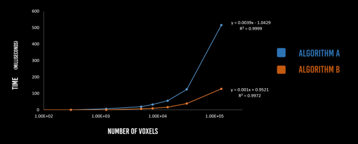
Figure 5. Display run-time as a function of the number of voxels
Software Seminar | MRAC 2018-2019
Guest Lecturer: Long Nguyen
MRAC Faculty: Eugenio Bettucchi
Student: Apoorv Vaish