HYPOTHESIS
The objective of this project is to explore the possibility of predicting the structural weight of a building given a massing model and column spacing.

METHODOLOGY
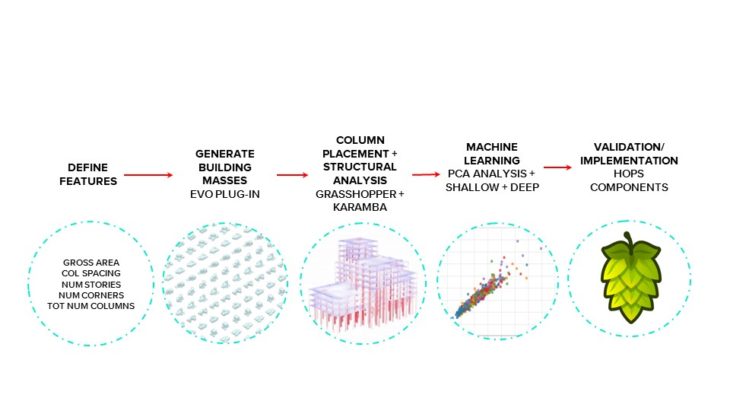
We approached this hypothesis using the following methodology:
- We begin by defining the structurally impactful features of a building.
- Then, we generate building masses in grasshopper using a plugin called Evo.
- Next we place the columns and run a structural analysis in Karamba. A grasshopper script records the data.
- The machine learning model trains on the dataset.
- Lastly, we bring the trained model back into grasshopper using hops for validation and visualization.
DEFINING FEATURES
Below, is one iteration of a building mass, showing all the features. The structurally impactful features identified are the following:
- Gross area
- Bbox width
- Bbox length
- Filling factor
- Num stories
- Num corners
- Perim. To area ratio
- Tot num columns
- Num overhang cols
- Overhang col length
Calculated features:
- Filling factor = volume / (bbox width x bbox length)
- Perim. To area ratio = overall perimeter / area

FEATURE SPACE // CREATION
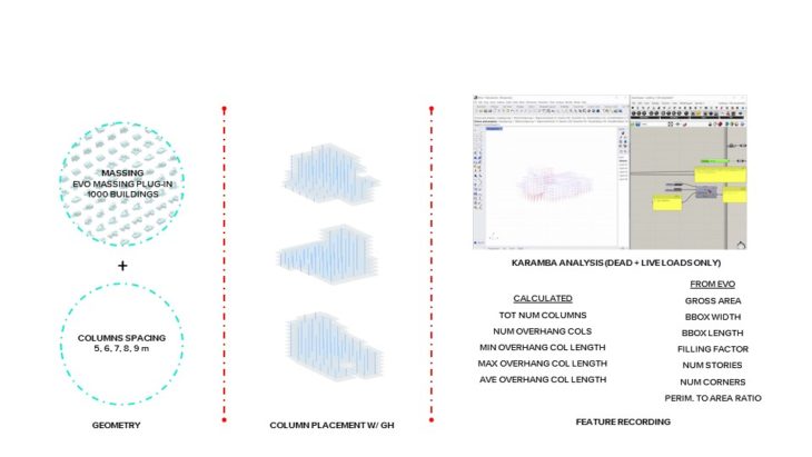
We generated 1000 building masses in grasshopper.
Next we place the columns at a spacing of 5, 6, 7, 8, and 9. Each building generated in Evo gets repeated 5 times with the different column spacings for a total of 5000 buildings.
Once the columns are placed, we run a structural analysis in Karamba on the 5000 buildings.
Our grasshopper script records the building features and their resulting structural weight.
DATA
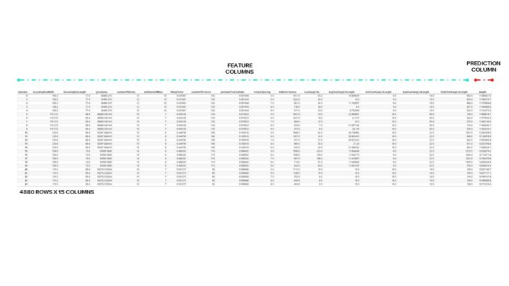
After dropping data points where data failed to be recorded, we ended up with 4,880 data points with 14 different features.
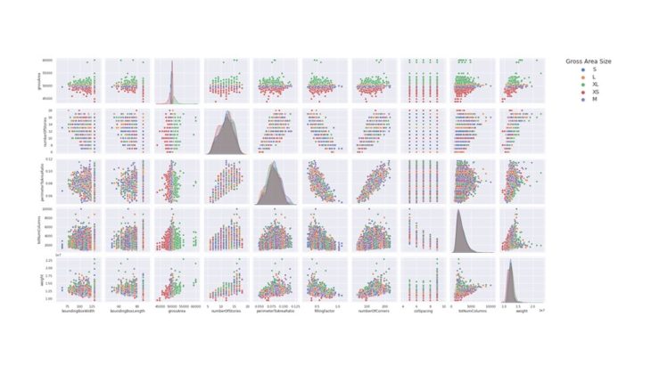
DATA VISUALIZATION // PAIR PLOTS
Plotting the features against each other, specifically looking at the last row, we begin to see a correlation between our features and weight.
DATA VISUALIZATION // CORRELATION MATRIX HEATMAP
Plotting the features against each other, we can see which ones are correlated. In our data set, the most correlated features are the perimeter to area ratio and number of corners.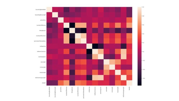
PCA // PRINCIPAL COMPONENT BIPLOT
This led us to a PCA analysis to see if there were any features that were just creating noise in our model and that could be removed. In this plot, we can see that bounding box width and bounding box length are the least influential on PC1 and PC2.
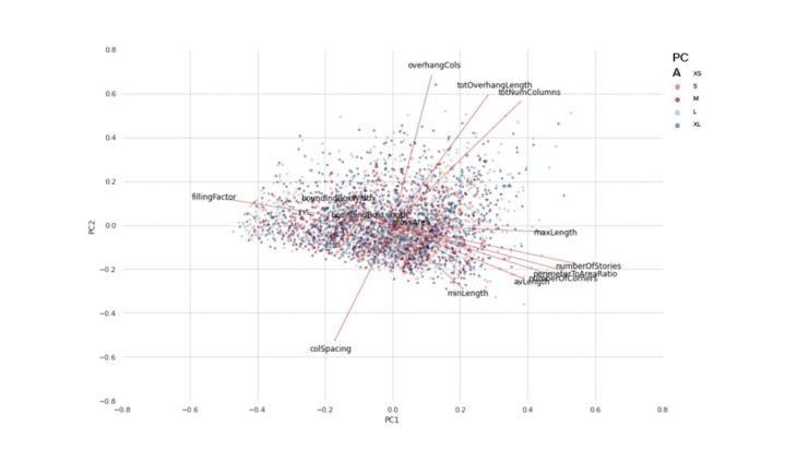
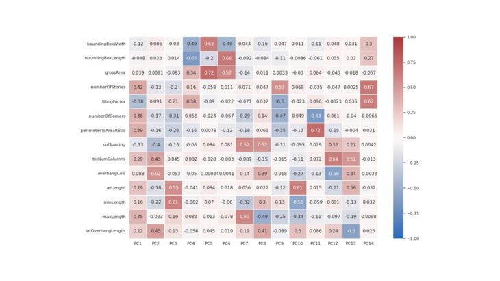
PCA // PRINCIPAL COMPONENT BIPLOT
This is further validated in the principal component biplot. We also learn that our most influential features are number of stories and the filling factor.
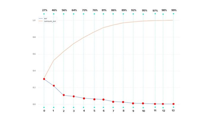
PCA // SCREE PLOT
However, when we plot the explained variance ratio on a scree plot we see that almost all of our principal components are required to capture the variance in our data. This indicates that the reduction of features via PCA analysis may not be a good technique to utilize.
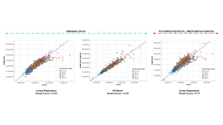
MODEL // COMPARISON
Comparing all the models, we see decent results with linear regression and improvement with XG Boost. As mentioned previously, we didn’t think that reducing features would be beneficial and this was validated when we saw worse results as we applied linear regression to a data set without the bounding box width and length. A trend we notice throughout is that all the models have a harder time predicting the weights of larger buildings. We will explore this further in the validation section.
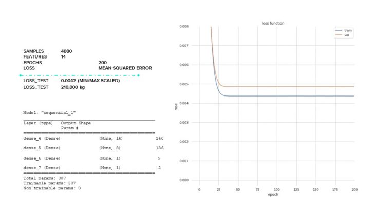
ANN // LOSS FUNCTION UNDERFITTING
Next, we tried an ANN model as we realized that our features were not necessarily linearly correlated to weight. We started off with a model with very few parameters, 387 and found that this was not enough parameters as our model displayed under fitting and was not able to learn the patterns of our data. We have a final loss value of 210,000 kg. Relatively speaking, considering our buildings have weights in the tens of millions, a mean squared error loss of 210,000 kg is not bad.
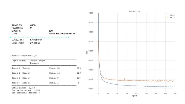
ANN // LOSS FUNCTION
However, we continued to experiment with the architecture of our model and found that increasing the density of our layers with a max number of total parameters of 1153 gave us a well fitting model with very small loss of 27,412 kg.
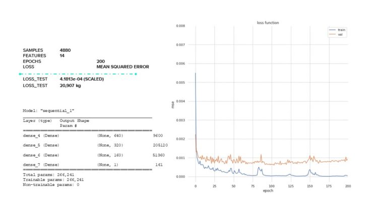
ANN // LOSS FUNCTION OVERFITTING
Lastly, we wanted to see what would happen if we made our architecture very dense. Even though we have the smallest loss value here out of all our models, we see when we plot our loss function that we have overfitting as the test loss values can be plotted almost exactly onto the train loss values.
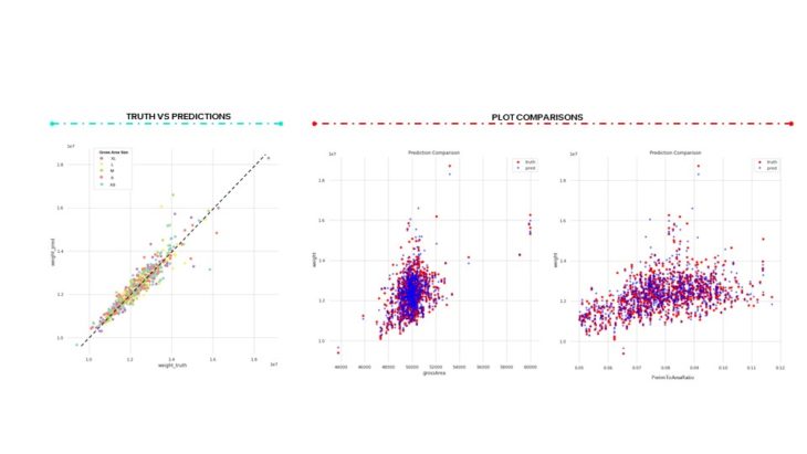
ANN // RESULT VISUALIZATION
Visualizing the results of our best ANN model, on the left we plot the real weight versus the predicted one. Again, like we saw with the shallow learning models, our model has more difficulty predicting the weights of larger buildings.
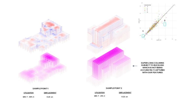
VALIDATION //VISUALIZE OUTLIERS
Next, we wanted to visualize a few of our outlier data points. Initially we hypothesized that Karamba wasn’t properly sizing the elements, which would have resulted in high utilization and displacement values. However, after looking at our results, we saw that this was not the case. But we did notice that a lot of our larger buildings masses generated by Evo had large overhangs resulting in super long, unrealistic columns that were affecting our weight, but whose features weren’t fully being represented in the model. If we were to do this again, we would first filter out the unrealistic building masses from our dataset.
VALIDATION // HOPS
Finally, we implemented our trained ANN model in a hops component with flask and ngrok to host and create an endpoint for the hops component. We liked this method as it allowed us to see in real time our building mass and the resulting predicted weight. At the same time, we also fed our building mass into our original Karamba model so that we could also compare the Karmaba weight to the predicted one.

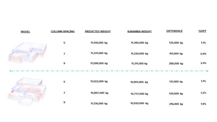
COMPARISON
Looking at the results from a couple of data points, we first noticed that across most of our buildings, a column spacing of 7 meters resulted in the lowest mass. This is what we originally thought would happen because when you have a small column spacing, you are over designing your building, but when your column spacing gets larger, your slab thickness must increase to compensate, increasing weight. As such, our predicted building weights were behaving as expected. Observing the percent difference between the real Karamba weight and the predicted weight, we see between a 1-2 percent difference, which, in the structural engineering world is amazing. To conclude, in terms of determining if we could generate a machine learning model to learn the patterns of our dataset, we were successful. However, we would not recommend using this model to predict building weights as it:
- was not generated on real buildings,
- did not include a lateral system or lateral analysis,
- was generated with Karmaba, which meant that we had to take a lot of short cuts and make a lot of assumptions in the structural modelling process that we wouldn’t otherwise take if we were trying to determine a buildings weight.
Overall, it was an interesting process to go through an entire supervised learning workflow in such a short amount of time.
CREDITS
STRUCTURAL WEIGHT PREDICTIONS WITH MACHINE LEARNING is a project of IAAC, Institute for Advanced Architecture of Catalonia developed at Master in Advanced Computation for Architecture & Design in 2021/22 by
Students: SOPHIE MOORE + AMANDA GIOIA
Faculty: GABRIELLA ROSSI + HESHAM SHAWQY