CONTEXT

Our term studio project ‘Drive in Nature’ asks the question; in a world without cars, what would happen to major motorways and junctions, and how could we utilise them to bring nature back into the city? The project is based in London, UK, and the surrounding metropolitan area. We focus on the fragmentation caused by human built infrastructure, the use of biodiversity as an indicator of ecosystem services, and how we can connect surrounding communities with the nature of the area they are living in. After analysing flows on Circuitscape and mapping land use in Greater London and surrounding areas, we decided to focus on a section of the A406 motorway near the Epping Forest. With this potential intervention area in mind, we needed to research the characteristics of the people and surrounding regions to understand what kind of repurposing would make sense in the area. Thus, we began gathering data from a variety of sources about the communities there.

DATA

The majority of the data used in our project has been publicly available in shapefile form. However, one of the challenges presented to us was needing to map data that was not properly geocoded. 

As part of our research for our proposed intervention on the selected area on the A406, we looked for data on socio-economic and demographic data on the communities in the area. This led us to the Consumer Data Research Centre (CDRC), which has a variety of spatial data (in CSV form) on demographics, health variables, accessibility metrics, etc. One of the indicators was ‘consumer vulnerability’, which is defined as a measure of how physically, mentally, and financially vulnerable a person is during a market interaction. The data was organized into six categories labelled from A to F based on these variables, with A as the lowest risk and F as the highest risk. Both these variables and the regions were defined based on 2011 Census data. Census data is organized by postal codes called the ONS Coding System and this particular dataset was coded by ‘Output Area’ (OA), which are regions of the smallest scale. Unfortunately, these in their CSV form have no geospatial qualities for mapping. 

The file we have for geolocated data is a shapefile published by the Office for National Statistics (ONS). It has many columns of different postal codes in the UK, but the relevant one to us is the 2011 OA codes, the same as in the consumer vulnerability CSV.

Thus, by merging the consumer vulnerability CSV and the geocoded shapefile through the common column of the OA codes, we obtain one dataset to be used to map the consumer vulnerability index. 

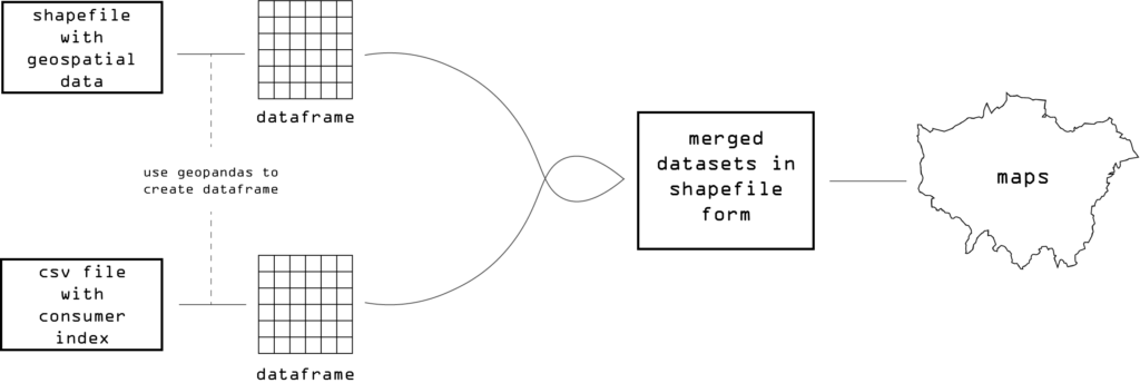
Flowchart of the dataset merging process

DIGITAL TOOLS & BIG DATA…SO FAR

The Digital Tools & Big Data I course has provided a solid foundation as an introduction to data science by using the Pycharm interface to learn the Python coding language. Starting from the basics of understanding environments and running basic commands, there has been a particular emphasis on learning about different types of data files and how to work with geospatial data in Python. An extremely powerful tool for data analysis, using Python for such has many advantages, including creating maps with large amounts of data, or writing code to create many maps quickly for a comparative analysis. For us, one powerful application of Python is using it to combine different file types to have geospatial data in a readable form. 

METHOD IN GEOPANDAS

Our first step is to import the ‘geopandas’ library, an extension of the ‘pandas’ library. Pandas is a library used to create data frames for statistical analysis, dividing the data into readable columns; geopandas incorporates all these features and adds the ability to work with geocoded data.

The next step was to read our geospatial data. We defined an object as the shapefile with the OA postal codes and created a dataframe by telling Python to read our object using geopandas; this gave us our first dataframe. The second step was similar to the first, to read our CSV file of consumer vulnerability. We defined an object as the relevant file with the consumer index and then created a dataframe. Note that this time we use ‘pandas’ to read the file because there is no geocoded data here. This will allow for easier merging of the files as the CSV will take the geo properties (e.g. CRS) of the shapefile.

After these two steps we have two dataframes, one with our location data and one with our consumer data, which share a common column of OA codes.

There were some issues with the naming of the columns; due to the shapefile having many columns of the ONS Codes themselves having some columns with overlapping characters, we needed to ensure we were merging by the correct column. For this, before merging, we made two updated dataframes where we specified that the column with the OA codes should only be read by the last six characters. After this process, we finally were able to correctly merge the files by running a line of code with the ‘merge’ command, specifying to merge the shapefile and the CSV by the last six digits of the previously defined column. Further, a line of code to print the column values was run to double check the process had been done correctly; finally, we could save the merged file as a shapefile by using the to.file command and defining the driver as an ESRI shapefile.

We use two methods for mapping; one map created in Python and two using the new shapefile in QGIS for further stylizing. The following map (Fig. 1) is generated in Python.

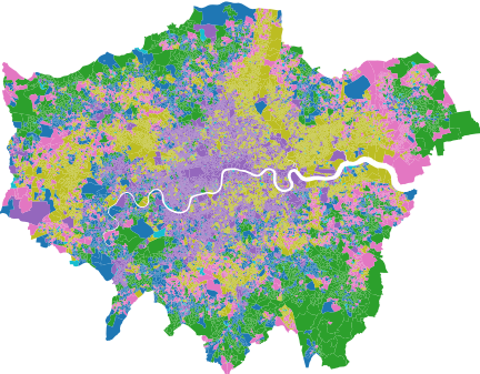
Fig. 1: Basic map of the consumer vulnerability index.

From this we understand a basic overview of the different clusters of consumer vulnerability in the city. For more detail and analysis, we used QGIS (Fig. 2.1 and Fig. 2.2).

Fig. 2.1: Our map of consumer vulnerability in Greater London; white indicates lower vulnerability and dark pink indicates higher vulnerability. Our indicator is a measure of financial, physical, and mental vulnerability during a market interaction as a consumer.

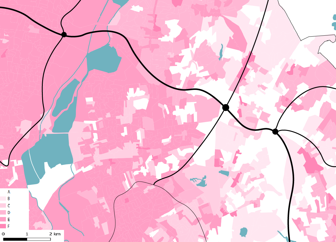
Fig. 2.2: This map shows the proposed intervention zone along the A406 motorway; we learn from the characteristics of the surrounding communities to inform us about what kinds of intervention would be beneficial. 

This process allowed us to map the area of our proposed intervention to further understand the community and the people in the surrounding area. From this map, we are able to determine that on the West side of our section is a more affluent and less vulnerable area, whereas on the East there is a higher risk neighbourhood. This has led us to propose an ecological corridor naturally extending from the edge of the Epping Forest and the lower risk area to connect with the higher risk area. We can extrapolate how creating an ecological corridor along this motorway to drive biodiversity back into the city and connect these two regions would be beneficial for the lower-income community; understanding these demographics is crucial for us to ensure we are proposing appropriate intervention. Learning the process of merging different files with Python allowed us to begin such analysis.

CONCLUSION

The process of learning how to merge CSV and shapefiles has proved very useful for us. We can now use data previously unable to be mapped to analyse the communities in the area and help develop the appropriate intervention zones for our term studio project. Moving forward, this process of combining files can be repeated for other indicators and will prove to be imperative as we continue to work with non-spatial data that needs to be represented visually.

Mapping Consumer Vulnerability is a project of IaaC, Institute for Advanced Architecture of Catalonia developed at Master in City and Technology, in 2021/2022 by:
Students: Joseph Bou Saleh, Dimitrios Lampriadis, Julia McGee, Kriti Nirmal
Faculty: Diego Pajarito