DAYLIGHTING PREDICTION FOR ATRIUMS:
LEED IEQ- Approach
“Atrium spaces have become a main part of most public buildings all over the world, regardless of their environmental aspects. The arguments of a good space, the psychological atmosphere and the impact on energy consumption are the main problems that face any designer, environmental designers in particular.”
THE PROBLEM: Simulation time and software
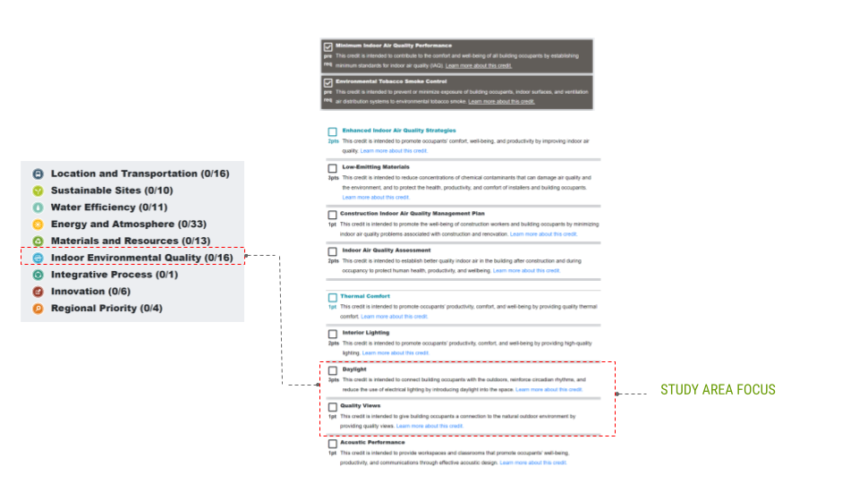
Atrium spaces globally form an integral part of many public buildings and have a great impact both psychologically and environmentally on the spaces they form. The ability to rapidly assess the physical form and environmental impact simultaneously while adhering to internationally recognized green building rating systems are invaluable in early-stage design. To fulfill indoor environmental quality (IEQ) requirements on green building rating systems like LEED, certain specifications are needed which can be time-consuming to calculate.
THE SOLUTION: AI Prediction
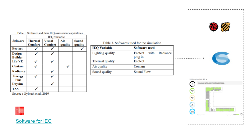
Choosing LEED green building Certification is for its reliability, in addition it is commonly used worldwide. Due to simulation time, The final results have focused on daylight autonomy, glare and quality view scores. Global environmental assessments like LEED, the ability to predict a score within seconds would be invaluable. For the purpose of this seminar we only focus on the daylight and quality as a starting point for this target.
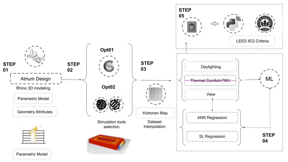
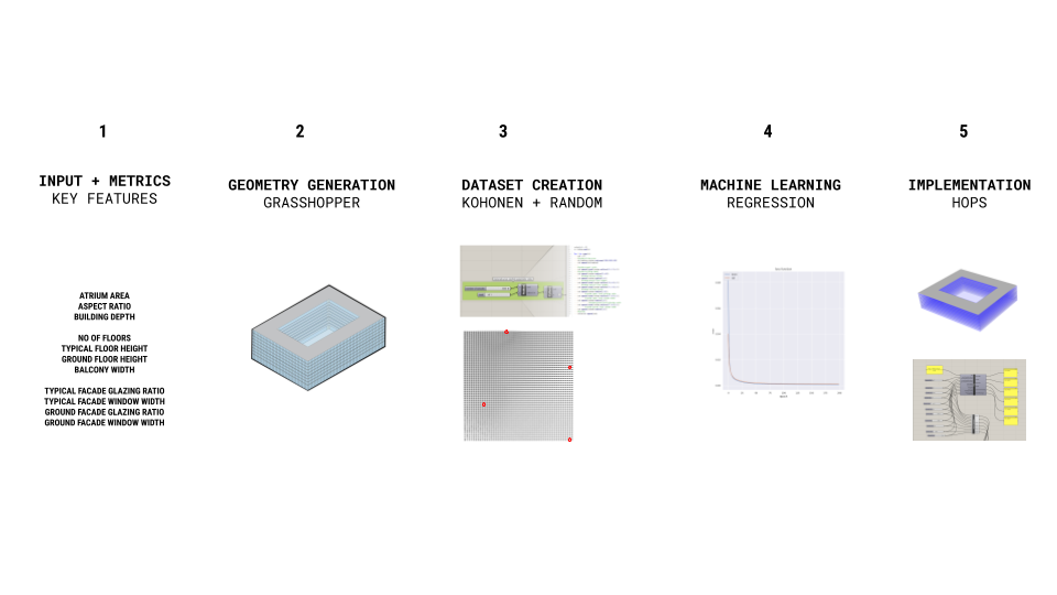
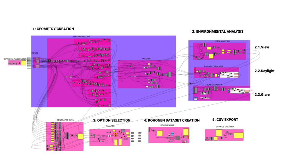
Our methodology relied on 5 main steps, the first is the geometric generative model, the second is the simulation tools, 3rd Kohonen map for dataset interpolation, 4th the ANN and SL AI model and finally prediction test on hops. There are five main steps in this workflow concluding with a live prediction using hops to translate the data into rhino and link it with the geometry.
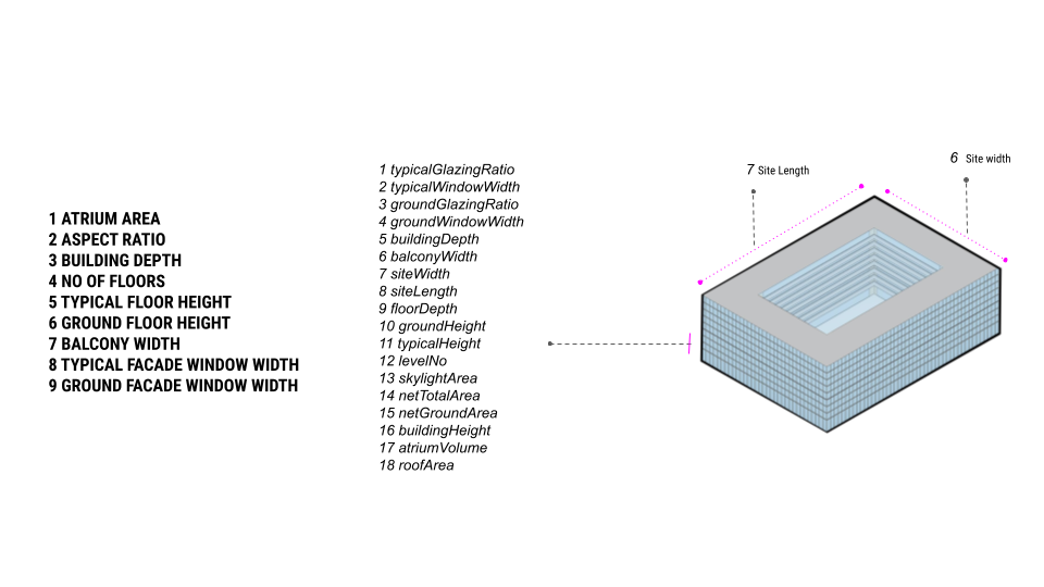
SCRIPTING, GEOMETRY, AND DATASET CREATION
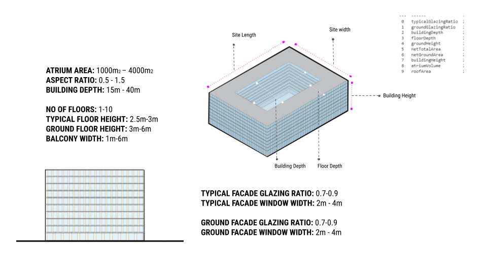
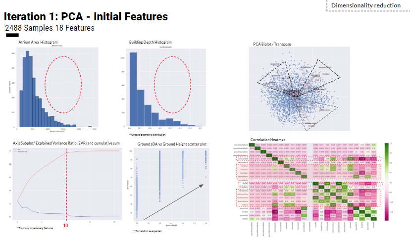
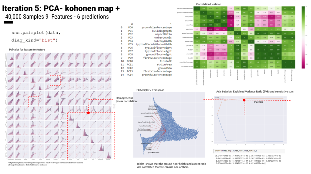
For the first step of deciding the main features which will be used for ML to predict the environmental analysis, we went through a process of reducing and refining the inputs from 18 features to describe our geometry to 9 features through dimensionality reduction through PCA. We trained our geometry on limits with these features for example min and max atrium areas and building depths.
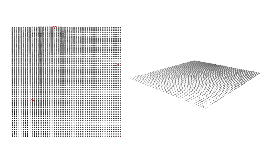
After the input selection, we explored 2 processes for data generation: one through a randomizer script. And the second method through using a Kohonen map using 4 extreme options chosen through the genetic optimizer Wallacei. This Kohnen map provided an interpolated dataset of any specified amount needed.
As for environmental simulation tools, two different tools are developed while a comparative analysis between results and simulation time has directed the team to adopt only one.
The Kohonen map interpolation is seeded with 8 seeds representing the minimum and maximum values of input features and predictions. 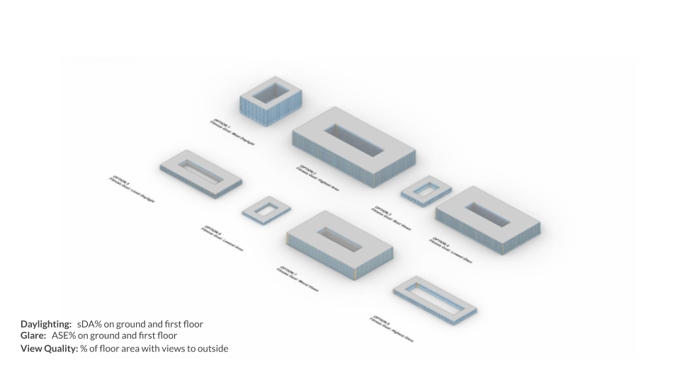
THE TRAINING: Dataset development and Regression
We tested 5 main iterations changing each time the regression model, predictions and features based on data analysis and PCA analysis. Two AI models have been examined, an ANN regression and a SL regression. ANN architecture for different datasets, simulation-sourced and Kohonen map-augmented, have been explored.
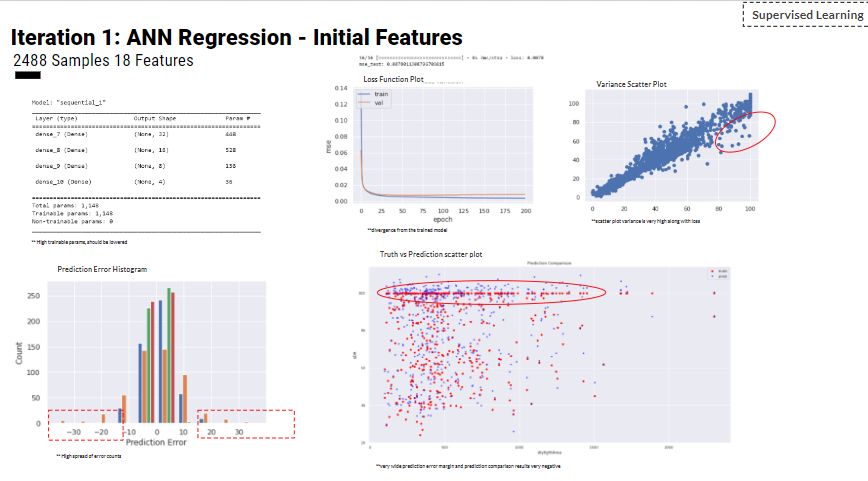
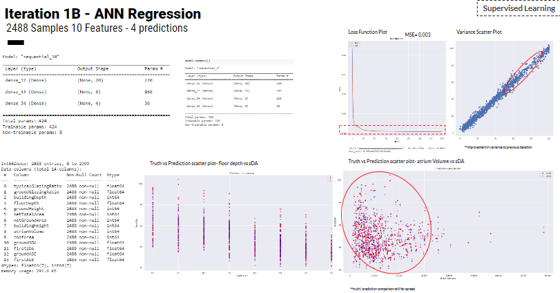
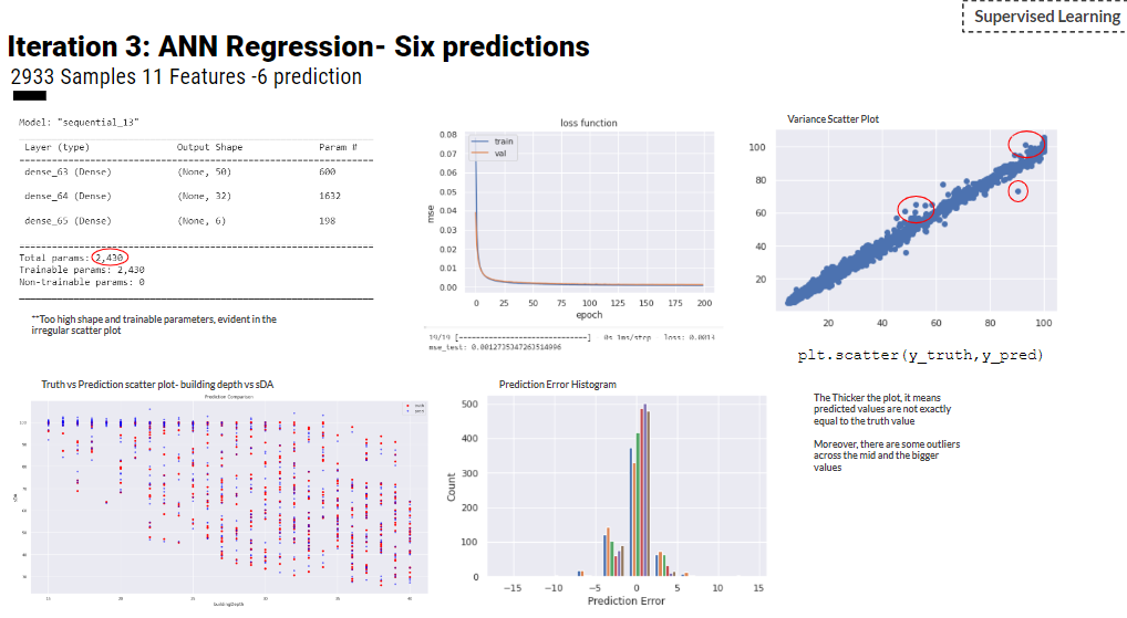
For the first iteration and analysis we could tell that the data was unevenly distributed and too many features, but could identify ones to remove through low correlation analysis such as balcony width, building height and various area features which duplicated information. Through initial testing with deep learning the prediction accuracy was very low due to inadequate dense layers and no clear features to correlate with the predictions this can be seen in the bottom right on the truth vs prediction plot.
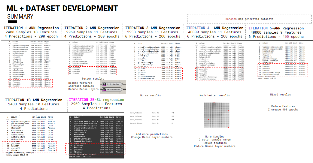
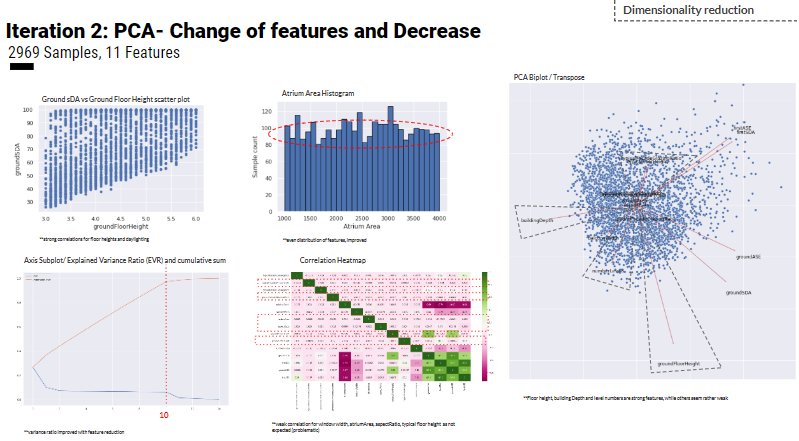
Basically, Iterations has been explored using different datasets, Iteration 1 to 3 used a dataset from a randomizer. While iterations 4 and 5 ran a Kohonen map interpolated dataset of 40, 000 samples. After dimensionality reduction with features in the 5th iteration, a minimum MSE loss function is achieved of 0.00016.
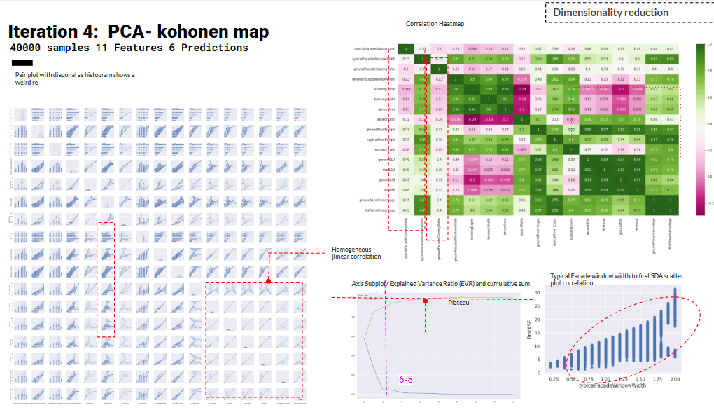
Over the iterations, we improved the geometry and features along with the sequential layers of the Regression model. For the 4th and 5th iterations we used the Kohnonen map as a way of increasing the sample size and to increase the interpolated steps between values for better correlations as seen the the heatmap and scatter plots. However, the covariance plot reached a plateau between 6-8 .
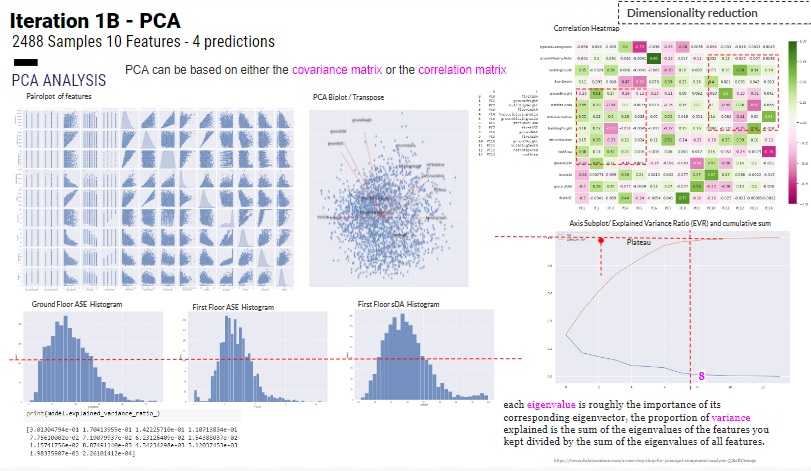
Iteration 1B has taken place after a dimensionality reduction of features from 18 to 10 features as per the results from the dataset PCA analysis. The MSE loss function is 0.003 which is improved model results from 0.007 of iteration 1.
Iteration 2
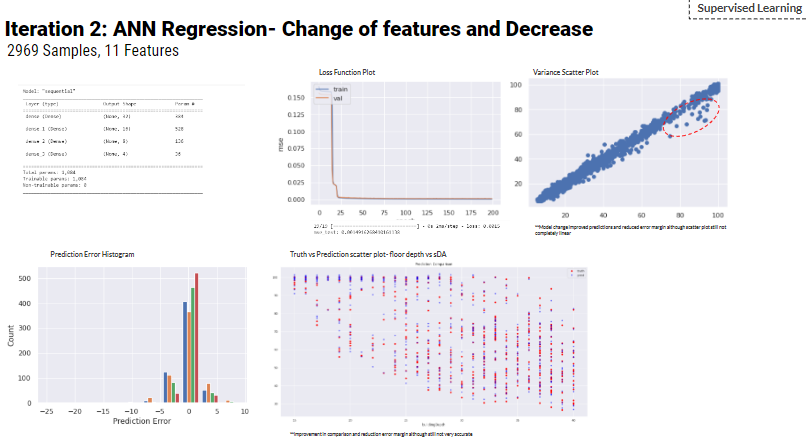
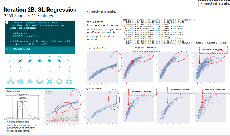
In Addition, the team has explored a different supervised learning algorithm, which is the Shallow linear learning regressions (SL regression) using 2969 samples (the same dataset for iteration 2) with 11 features to predict daylight autonomy of atrium buildings.
The SL regression uses a standard scalar of the dataset to improve the model results. However, the train versus prediction graphs shows a polynomial correlation rather than a linear one. Hence, the team decided to train more ANN.
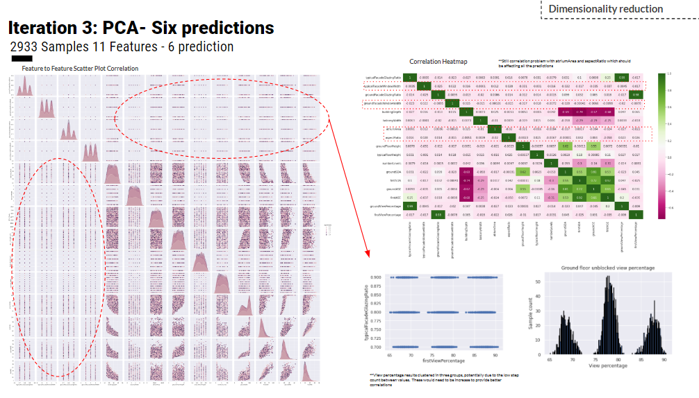
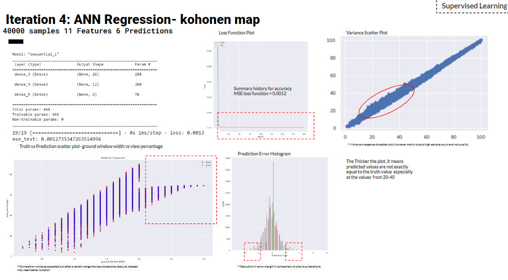
In iteration 3, another prediction is added which is the quality view to meet LEED-IEQ scoring categories. Basically, 11 features are used to train ANN regression for 6 prediction. The MSE loss function is 0.0012. However, the covariance scatter-plot shows some outliers so we decided to increase the dataset size and train more.
Hence, In iteration 4 and 5, a Kohonen map interpolated dataset of 40,000 samples is used to train ANN regression. PCA analysis of features in the covariance EVR plot has reached a plateau of nearly 8. So, the team trained a model of the 11 features for iteration 4 . While a dimensionality reduction has taken place to train iteration 5.
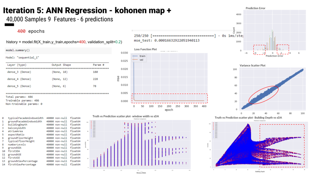
Iteration 5 uses a 40000 sample dataset and is trained with an ANN regression model with 3 dense layers of 36 neurons using ‘relu’ as an activation function, ‘Adam’ as an optimizer, and ‘mean_squared_error’ as a loss function. Finally, Hops is used to visualize and test. Finally, results show successful predictions of values within the min/max used to train the models.
As a result of dimensionality reduction to 9 features, in iteration 5 ANN regression. Moreover, the model is trained with double hyperparameters of 400 epochs. Consequently, an optimum result of the MSE loss function reaches 0.00016 which is the minimum of all iterations.
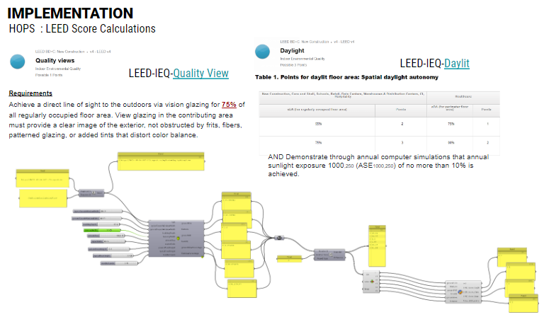
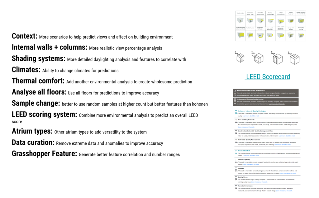
IMPLEMENTATION: Hops and LEEDs Scoring
The final step involved implementing the ML model for prediction through hops to connect to live geometry in rhino and show real-time environmental analysis instantly.
A script was added to convert the predicted analysis into a LEEDs score category and assign the points accordingly. hops is used for the prediction test. In addition, we added a script for leed IEQ points calculation using iteration 5 trained ANN regression model. If the view percent is 75 or more we gain 1 point. For daylight, from 55 to 75 we gain 2 points. With more than 75 we gain 3 points. As for the ASE or glare, it should be less than 10 %.
Future Work
After running all these iterations we learned a lot about the process to create better predictions. To further develop this project we would rework the original grasshopper script to improve the features, and ranges and add more influential geometry such as walls and facades. In addition, We would hope to add further analysis to provide rapid LEEDS evaluations with the rest of the criteria.
STUDENTS: MICHAL GRYKO + SAMMAR ALLAM
SENIOR FACULTY: GABRIELLA ROSSI
FACULTY ASSISTANT: HESHAM SHAWQY
COURSE DIRECTOR: DAVID ANDRES LEON