The project AIR QUALITY 3D MAPPER was developed during the S2 Software II Seminar of the MRAC 2020/21 program.
Overview
An estimated 3.4 million people died prematurely as a result of outdoor air pollution in 2017. This means that outdoor air pollution was responsible for 6% of global deaths. In 2016, household air pollution was responsible for 3.8 million deaths, and 7.7% of the global mortality.
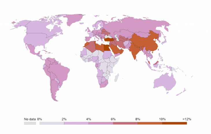
link to credits for image above
Our project proposal for this seminar was to scan an interior space and to visualize the air quality data in order to potentially introduce architectural solutions that could help enhance the indoor air quality.
Hardware
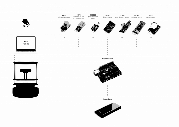
In order to scan, we used a Turtlebot 2 along with a lidar scanner. We were able to visualize our scan using ROS (Robotic Operating System) and control the turtlebot within the context by localizing using SLAM (Simultaneous Localization and Mapping). We were working on ROS Melodic and therefore had to use the turtlebot2 package and lidar package that was compatible. Along side the turtlebot, we also used a set of sensors to collect and evaluate air quality data.
GMAPPING
We selected three main spaces in P59 to collect data; the laser cutting area, studio space 1, and the hallway in between the two spaces mentioned above. The visualization of the maps for the hallway and space 1 were done using hector gmapping rviz file (the package can be found in the github), and the visualization of the map for the laser room was done using a modified launch file.
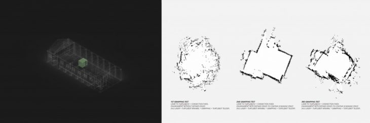
HALLWAY
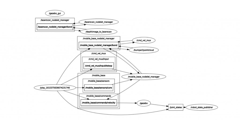 Gmapping node diagram of the hallway
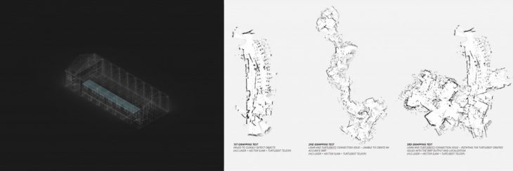
The hallway is a common area with several students and professors walking through, which meant that we would have some difficulties making an accurate map. However, there were more technical problems when producing the three maps shown above. In this first try, the lidar scan topic and the turtlebot transformation topic were not subscribing to a final topic. As can be seen in the node diagram, the laser scan is on its own and the joint states of the turtlebot are also on its own therefore, we were not able to create an accurate map since there was no communication between the lidar and the turtlebot. This was mainly due to the fact that we launched the turtlebot and lidar separately, but had not made a file that would launch them simultaneously. This created a disconnect between the two topics therefore creating a map using the lidar but not being to use the odometry for localization.
SPACE 1
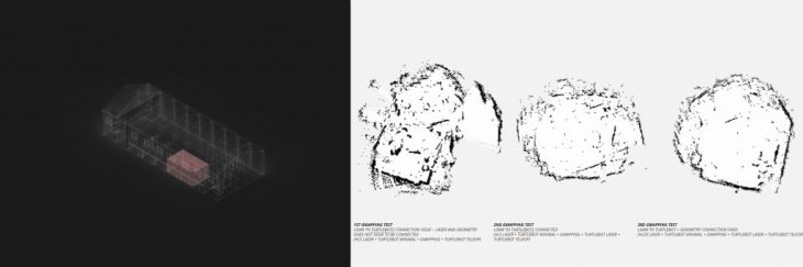
Scan of studio Space 1
We first took a photogrammetric scan of space one and created a dense point cloud in order to have a generic layout of the space.
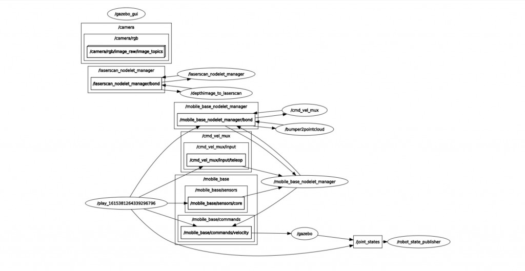
Gmapping node diagram of studio Space 1
The studio space is more defined by walls, in comparison to the openness of the hallway, therefore it resulted in cleaner maps. We made a launch file to connect the lidar and turtlebot topics yet the node diagram above still shows a disconnect between the two.
LASER CUTTING AREA
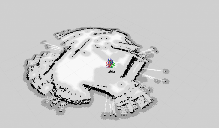
Scan of Laser Cutting Area
We then moved to the laser cutting space. We put up cardboard walls and created a strict boundary around the space that we scanned. We then updated the launch file in order to properly subscribed to the topics scan and tf (transforms). These launch files and the rest of the packages for the lidar and turtlebot 2 can be found in the GITHUB.
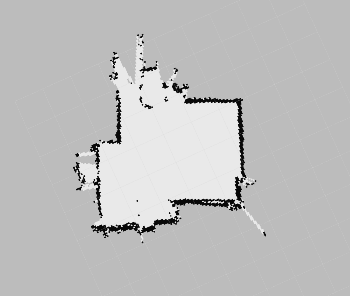
Final map output of laser cutting area
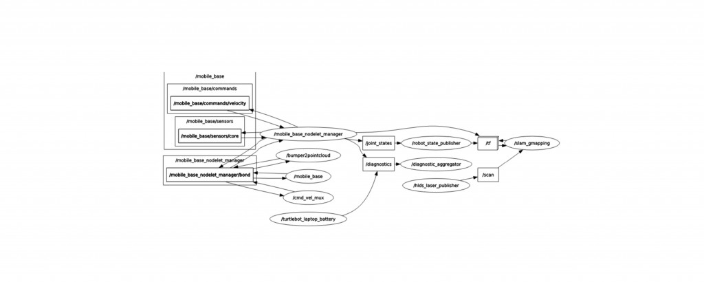
Gmapping node diagram of the laser cutting area
After reviewing the errors and debugging the launch files, we noticed that the node diagram output had the necessary topics subscribing to both the turtlebot tf (transforms) and the lidar scan. This resulted in a that can be used for AMCL (localization system for a robot moving in 2D).
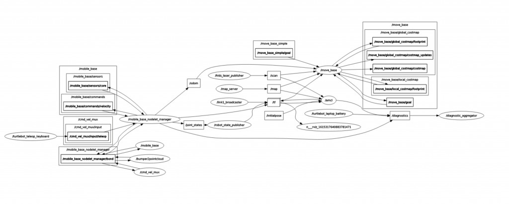
AMCL node diagram of the laser cutting area
The node diagram above clearly indicates that we are able to visualize all of the move base topics, which allows us to navigate the turtlebot in a known environment aware of its surroundings. The costmap (as shown below) outputs a map with buffer zones for the turtlebot to be aware of and in return the turtlebot is not able to go those zones, and it is able to freely navigate outside of those zones.
The costmap includes an offset of the walls/ objects that the lidar scan has detected, but it also works in real time to detect any other moving things. The zones where there are no walls/ objects (black lines) present were where we were standing to test how well we were receiving information with the scanner in real time.
Air Quality Data Collection
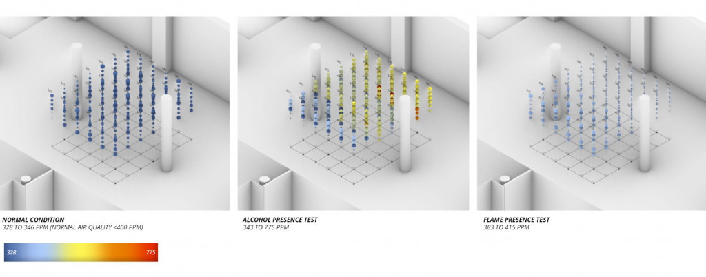
Normal Condition
The first data collection was used as a reference to measure air quality, taking the data from a space without any particular condition. With this data we establish a ‘regular’ scenario.
Alcohol Presence Test
The second data collection shows a different scenario where the air was modified with alcohol. This allows us to understand and also visualize the changes in the values ??of the gas sensor mq 135.
Flame Presence Test
The third data collection shows the third scenario which was a space intervention with the presence of a flame.
The three data collection campaign allows us to understand and visualize the data we are dealing with. The base measure for normal air quality was between 350 and 400 ppm. When we modify the air quality scenarios, we obtain measurements above 700 ppm.

AIR QUALITY 3D MAPPER is a project of IaaC, Institute for Advanced Architecture of Catalonia developed at the Master of Robotics and Advanced Construction program in 2020/21 by:
Students: Helena Homsi, Juan Eduardo Ojeda, Aslinur Taskin
Faculty: Carlos Rizzo
Faculty Assistant: Soroush Garivani